The WXYZ Model - Step 3

Now that we have designed our deterministic model, we can use most of the same code to produce a probabilistic output. This is one of the key reasons why it’s useful to have specified our functions ‘get_values’, ‘make_matrix’, and ‘make_cea’. Because these functions all feed into each other, the key additional step is to re-specify the object ‘df_values’ that stores our parameter values, then re-run the rest of the model on a loop.

After we have loaded our packages and functions, defined our controlling parameters, and imported our model inputs, we are going to create some blank objects to hold data: arrays to hold our Markov trace for all simulated runs, and dataframes to hold our costs and QALYs.

# Arrays to hold the Markov trace outputs
  mtraceout_trt <- mtraceout_notrt <- array(0, dim = c(n_t+1, n_states, n_sim))

# Dataframes to hold the CEA results
  df_c <- df_e <- as.data.frame(matrix(0,
                               nrow = n_sim,
                               ncol = n_str))
  colnames(df_c) <- colnames(df_e) <- v_names_str

Now we set up our loop to perform the probabilistic analysis. Each loop completes the following steps:

1. create the Markov trace matrix
2. load a set of probabilistic parameter estimates with ‘get_values’
3. populate the transition matrix with ‘make_matrix’
4. run the Markov model
5. calculate costs and QALYs with ‘make_cea’
6. record outputs

# 'n_sim' probabilistic values are stored in a dataframe called 'df_values'
df_values <- varlist$df_psa_input

# Set number of probabilistic simulations
n_sim <- 1000

# Calculate 'n_sim' probabilistic simulations of the Markov output
for (j in 1:n_sim){
  # 1 - Create the markov trace matrix
    m_M_notrt <- m_M_trt <- matrix(NA, 
                                    nrow     = n_t + 1, ncol = n_states,
                                    dimnames = list(paste("cycle", 0:n_t, sep = " "), v_n))
  
  # 2 - Load a set of probabilistic parameter estimates with 'get_values'
    # Take the values from row 'j' of the list of parameter values
    list_values <- get_values(df_values[j,])
  
  # 3 - populate the transition matrix with 'make_matrix'
    # calculate the transition matrices based on the values in 'list_values'
    list_tmatrix <- make_matrix(list_values)
  
  # 4 - run the Markov model
    # Populate the first row of the transition matrix
    m_M_notrt[1, ] <- m_M_trt[1, ] <- c(list_values$p_W, list_values$p_X, 0, 0, 0, 0)
    # Loop through the number of cycles
    for (t in 1:n_t){
      # Estimate the Markov trace for each cycle 't'
      m_M_notrt[t + 1, ] <- t(m_M_notrt[t, ]) %*% list_tmatrix$m_P_notrt
      m_M_trt[t + 1, ]    <- t(m_M_trt[t, ])  %*% list_tmatrix$m_P_trt      
    }
  
  # 5 - calculate costs and QALYs with 'make_cea'
    cea_out <- make_cea(list_values, m_M_notrt, m_M_trt, v_dwe, v_dwc)
    
  # 6 - record outputs
    mtraceout_notrt[,,j] <- m_M_notrt
    mtraceout_trt[,,j]   <- m_M_trt
    df_c[j,]             <- cea_out$Cost
    df_e[j,]             <- cea_out$Effect
  
  } # End loop

The loop is taking parameter data from the ‘df_psa_input’ object that is stored within the ‘varlist’ object created by the Batch Importer. Each row in ‘df_psa_input’ contains a probabilistically sampled set of parameter values. I am still using ‘j’ to denote the simulation number within each loop, which corresponds to the row number in ‘df_values, which is a copy of ‘varlist$df_psa_input’. As we loop through each step, the code adds a slice to each array and a row to each dataframe until it has computed these values ‘n_sim’ times.

My machine takes only a couple of seconds to perform this loop 1,000 times. This is faster than the array-based method, albeit not noticeably at such a small number of simulations.

The last part of this process is to view our results, calculated using ‘dampack’. There are lots of results that someone might be interested in, but I think a pretty common set of things you’d want to see from your model is:

• the mean and incremental costs and QALYs for each strategy, along with the mean ICER
• probability of cost-effectiveness at different levels of willingness to pay for a QALY (lambda)
• probability of cost-effectiveness at our baseline estimate of societal lambda
• the cost-effectiveness acceptability curve (CEAC)

So let’s find those. First we’ll need to create the kind of object ‘dampack’ uses to store PSA results. Then we can summarize the mean and incremental costs and mean ICER using the ‘calculate_icers’ function in ‘dampack’ and the outputs we recorded from the model in the last section of the code.

# Create a PSA object
l_psa <- make_psa_obj(cost          = df_c, 
                      effectiveness = df_e, 
                      parameters    = df_values, 
                      strategies    = v_names_str)

# Mean and incremental costs/QALYs, mean ICER
psa_sum <- summary(l_psa, calc_sds = TRUE)  # Estimate the mean costs, QALYs  
df_cea <- calculate_icers(cost       = psa_sum$meanCost,
                          effect     = psa_sum$meanEffect,
                          strategies = psa_sum$Strategy)

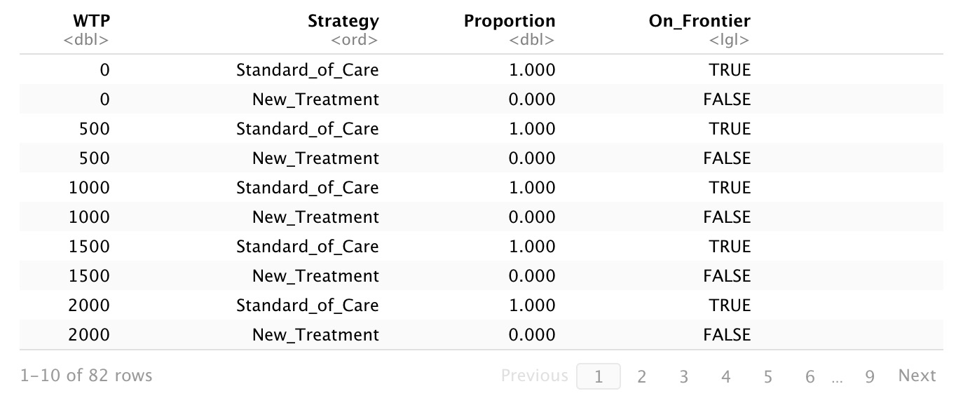
Having done that, we want to know what strategy we should choose at various levels of lambda. There are lots of different ways to present this information, so I just arbitrarily chose to look at a range of values from 0 to 200% of lambda in increments of 5% of lambda. This gives us 41 values, which is enough to suggest the shape of the curve. The smaller the increments, the more points on your curve. From there we can use the ‘ceac’ function in ‘dampack’ to generate estimates of probability of cost-effectiveness at our various values of WTP, including lambda. We can pull out the middle estimate of those probabilities to get the value at lambda for the new treatment.

# Calculate percent cost-effectiveness of each strategy
v_wtp        <- seq(0,2*lambda, by = lambda/20) # Vector of WTP values from 0 to 2*lambda
ceac_obj     <- ceac(psa = l_psa, wtp = v_wtp)
summary_ceac <- summary(ceac_obj)

# Calculate probability that new treatment is cost-effective at lambda
n_midwtp       <- length(v_wtp)+1            
n_trtPercentCE <- 100*ceac_obj$Proportion[n_midwtp]  

Let’s check out our results.

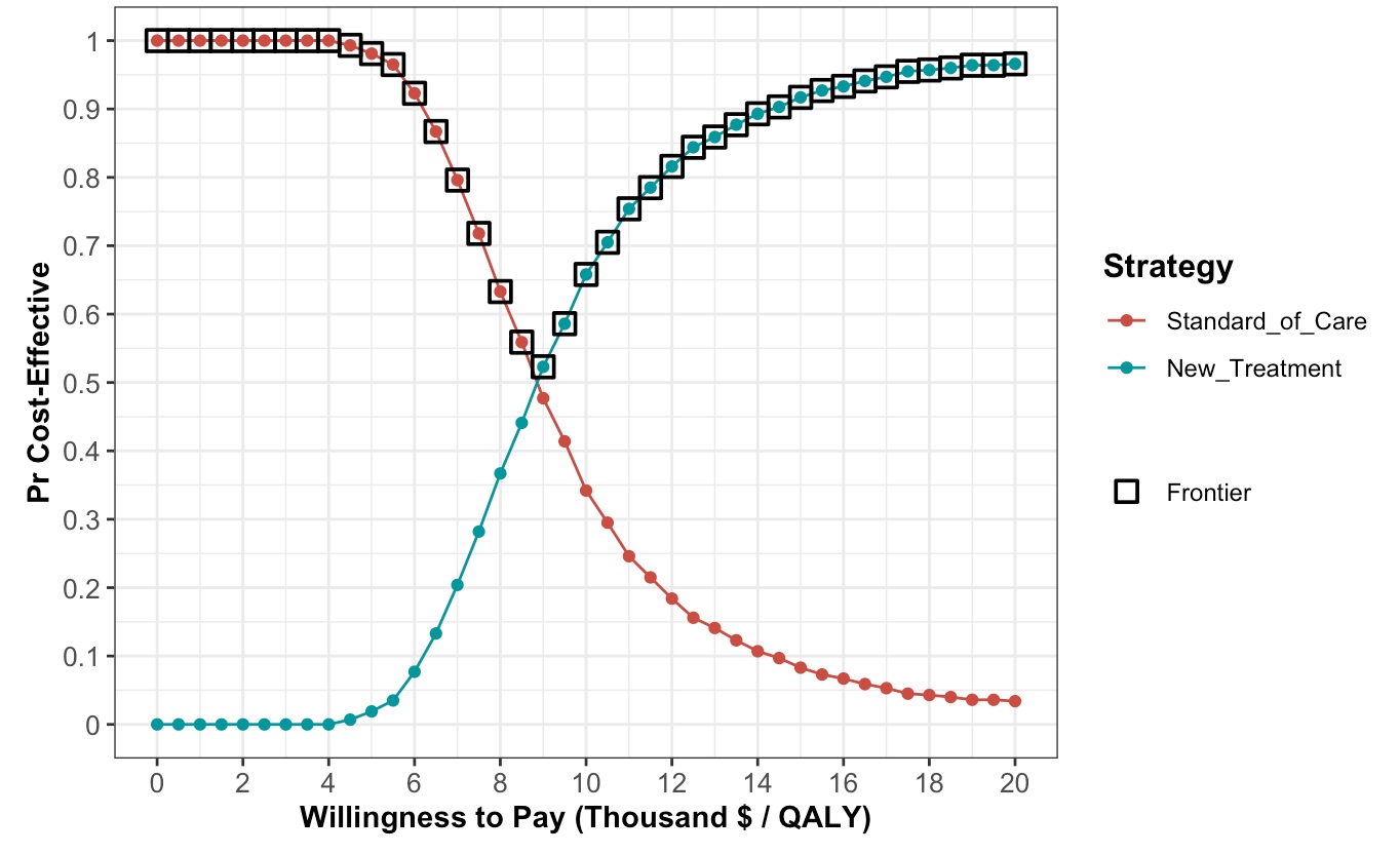
Our new treatment generates an additional 0.57 QALYs at a cost of just under $5,000 per person (ICER = $8840 per QALY). If we think society is willing to pay $10,000 per QALY,¹ there is a 65.8% probability that we would consider it cost-effective to fund the new treatment.

Back to top

Back to Step 1

Back to Step 2