If you’ve never built a function in R before, the process is less complicated than it seems. I’ve written up a quick summary with a simple example.
Function 1: “get_values”
The first function we are going to write is called “get_values”. This function takes one input ‘invals’, which is the output of the Batch Importer and contains all the user-defined input values. The function takes these inputs and converts them into parameters (remember my shorthand: inputs live in Excel, parameters live in R). Since some of our parameters are derived from input values (i.e., our ‘returning’ probabilities, our treatment-adjusted transition probabilities), we will use “get_values” to calculate these as well. You’ll recognize most of this from Chapter 4.4, except now we are using the Batch Importer.
# Read in parameters using Batch Importer
source("ImportVars.R")
Inputs <- read_excel("Model Inputs.xls") #The Excel file name
Inputs <- subset(Inputs, Value >-1) #Remove blank rows
varlist <- ImportVars(Inputs, n_sim)

# Specify a dataframe of parameter values
df_values <- data.frame(varlist$varmean)
colnames(df_values) <- varlist$varname
Now we tell R where to find the parameter values within our list of inputs (‘invals’).
get_values <- function(invals){
  # An empty list to hold data
  outvals <- list()

  # Transition probabilities (per cycle)
  outvals$p_WtoX        <- invals$P_WtoX
  outvals$p_XtoW        <- invals$P_XtoW
  outvals$p_XtoY        <- invals$P_XtoY
  outvals$p_YtoZ        <- invals$P_YtoZ

  # Other probabilities
  outvals$p_W           <- invals$P_W

  # Cost and utility inputs
  outvals$c_W           <- invals$C_W
  outvals$c_X           <- invals$C_X
  outvals$c_Ytransition <- invals$C_Ytransition
  outvals$c_Y           <- invals$C_Y
  outvals$c_Ztransition <- invals$C_Ztransition
  outvals$c_trt         <- invals$C_trt

  outvals$u_W           <- invals$U_W
  outvals$u_X           <- invals$U_X
  outvals$u_Y           <- invals$U_Y

  # Define returning probabilities
  outvals$p_Wreturn     <- 1 - outvals$p_WtoX
  outvals$p_Xreturn     <- 1 - (outvals$p_XtoW + outvals$p_XtoY)
  outvals$p_Yreturn     <- 1 - outvals$p_YtoZ
  outvals$p_X           <- 1 - outvals$p_W
I’ve added a function to the Batch Importer that allows us to convert back and forth between rates and probabilities (‘PtoR’ and ‘RtoP’ respectively), since we are now using a Rate Ratio to describe the effect of treatment. This requires us to do a slightly new calculation to derive the treatment-adjusted probability of transition from X to Y:
# Treatment-specific probabilities
RR_trt         <- invals$RR_Treat           # RR of treatment
XtoYrate       <- PtoR(outvals$p_XtoY, 1)   # convert probability to rate
rate_XtoYtreat <- XtoYrate*RR_trt           # calculate rate under treatment
prob_XtoYtreat <- RtoP(rate_XtoYtreat, 1)   # convert rate to probability
What we do in these steps is to convert the transition probability into a rate, apply the relative rate (RR) of treatment, then convert that back into a transition probability.1
“get_values” will return a list (referred to as ‘outvals’ within the function) of named parameters that we can refer to in the subsequent steps of the model.
# An empty list to hold data
outvals <- list()

outvals$p_XtoY_trt    <- prob_XtoYtreat
outvals$p_Xreturn_trt <- 1 - (outvals$p_XtoW + prob_XtoYtreat)

return(outvals)
}
Function 2: “make_matrix”
The biggest difference between my approach and the DARTH approach is that while I specify each transition individually, the DARTH method makes use of a transition matrix. A transition matrix is a description of the relationship between different states from cycle to cycle. If properly done, these two approaches will produce the same result. The matrix-based approach, however, is a lot faster in terms of R’s processing power. Plus it happens to be a lot closer to other acknowledged standard approaches. So since I’m not smarter than everyone else, I’m not going to ask you to do things my way.
“make_matrix” takes one input ‘paramlist’, which is the parameter list produced by “get_values”. The Markov matrix will have a number of rows and columns that is equal to the number of health states, and each cell within the matrix will contain the transition probability from one state (rows) to another (columns) - this includes the “returning” states.
Here’s a quick illustration:
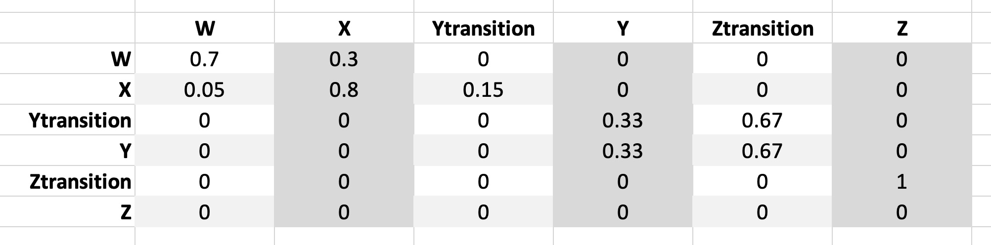
So here we see that the transition probability of going from State W to State X (for example) is expressed where row W meets column X. We can also see that the transitions between X and Y (and Y to Z) are actually transitions into our “Ytransition” state. Since the transition probability to Z (again, actually Ztransition) is assumed to be the same for everyone in the Y state, both Ytransition and Y have the same transition probabilities. All cohort members in Ztransition move to Z, and all members in Z stay in Z.
v_n          <- c("W", "X", "Ytransition", "Y", "Ztransition", "Z")  # health state names
n_states     <- length(v_n)         # number of health states

# create the transition probability matrix for NO treatment
m_P_notrt  <- matrix(0,
                     nrow = n_states,
                     ncol = n_states,
                     dimnames = list(v_n, v_n)) # name the columns and rows of the matrix
We start with a vector of health state names. We’re going to use it to create an empty matrix for our model arm representing standard of care (“notrt”). Next we’re going to populate that matrix with the transition probabilities from our ‘paramlist’ input.
# from W
m_P_notrt["W", "W"  ] <- paramlist$p_Wreturn
m_P_notrt["W", "X" ]  <- paramlist$p_WtoX

# from X
m_P_notrt["X", "W" ]             <- paramlist$p_XtoW
m_P_notrt["X", "X"]              <- paramlist$p_Xreturn
m_P_notrt["X", "Ytransition"]    <- paramlist$p_XtoY

# from Y
m_P_notrt["Ytransition", "Y"]             <- paramlist$p_Yreturn
m_P_notrt["Y", "Y"]                       <- paramlist$p_Yreturn
m_P_notrt["Ytransition", "Ztransition" ]  <- paramlist$p_YtoZ
m_P_notrt["Y", "Ztransition"]             <- paramlist$p_YtoZ

# from Z
m_P_notrt["Ztransition", "Z"  ] <- 1
m_P_notrt["Z", "Z"  ]           <- 1
Next we’ll make the transition matrix for our model arm representing the cohort receiving the new treatment. Since our two model arms have the same health states, we can just make a copy of “m_P_notrt” and then add in the different values that relate to the new treatment.
# create transition probability matrix for treatment same as no treatment
m_P_trt <- m_P_notrt

# add treatment effect
m_P_trt["X", "X"]            <- paramlist$p_Xreturn_trt
m_P_trt["X", "Ytransition" ] <- paramlist$p_XtoY_trt
Finally, we’re going to store our two transition matrices in a list. The function returns that list.
mtxout$m_P_notrt  <- m_P_notrt
mtxout$m_P_trt    <- m_P_trt

return(mtxout)
Function 3: “make_cea”
Finally we’ll need a function that takes a completed Markov trace, applies the cost and utility parameters, and then calculates LYG, QALY, and total costs for each arm. That function, “make_cea”, takes five inputs:
- paramlist: a list of probabilistically-sampled parameters from ‘getvals’
- mtx_trt: the Markov trace for the ‘trt’ arm
- mtx_notrt: the Markov trace for the ‘notrt’ arm
- disc_o: the discount rate for outcomes
- disc_c: the discount rate for costs
We’ll start by creating vectors that contain our estimates for cost and utility, corresponding to each health state:
make_cea <- function(paramlist, mtx_notrt, mtx_trt, disc_o, disc_c){
  # Vector of utility weights
    v_u_notrt <- v_u_trt  <- c(paramlist$u_W,
                               paramlist$u_X,
                               paramlist$u_Y,
                               paramlist$u_Y,
                               0,
                               0)

  # Vector of costs - 'notrt' arm
    v_c_notrt   <- c(paramlist$c_W,
                     paramlist$c_X,
                     paramlist$c_Ytransition,
                     paramlist$c_Y,
                     paramlist$c_Ztransition,
                     0)

  # Vector of costs - 'trt' arm
    v_c_trt     <- c(paramlist$c_W,
                     paramlist$c_X + paramlist$c_trt,
                     paramlist$c_Ytransition,
                     paramlist$c_Y,
                     paramlist$c_Ztransition,
                     0)
There are no differences between the utility of the ‘notrt’ and ‘trt’ arms, so we can create them both in the same command. We have to create different cost vectors for each arm because there is our treatment cost that is associated with being in “X”.
With that done, we perform our matrix calculations for costs and utilities, and export values to a dataframe called ‘df_ce’.
  ## Calculate mean Costs and QALYs for Treatment and NO Treatment
    v_tu_notrt  <- mtx_notrt   %*%  v_u_notrt
    v_tu_trt    <- mtx_trt     %*%  v_u_trt

    v_tc_notrt  <- mtx_notrt   %*%  v_c_notrt
    v_tc_trt    <- mtx_trt     %*%  v_c_trt

  ## Calculate Discounted Mean Costs and QALYs
    tu_d_notrt  <- t(v_tu_notrt)   %*%  disc_o
    tu_d_trt    <- t(v_tu_trt)     %*%  disc_o

    tc_d_notrt  <- t(v_tc_notrt)   %*%  disc_c
    tc_d_trt    <- t(v_tc_trt)     %*%  disc_c

  # store them into a vector
    v_tc_d      <- c(tc_d_notrt, tc_d_trt)
    v_tu_d      <- c(tu_d_notrt, tu_d_trt)

  # Dataframe to hold outputs
    df_ce       <- data.frame(Strategy = v_names_str,
                              Cost     = v_tc_d,
                              Effect   = v_tu_d)
  return(df_ce)
}
We are going to use these functions to make the model run both Step 2 and Step 3.
-
The code uses ‘1’ as the second argument in the rate/probability conversion functions. This input is needed for the function to work for reasons that aren’t terribly important. I would strongly suggest that when you add your values to the model, you convert the value of rates and probabilities to match your cycle length. ↩