The WXYZ Model

The first step we need to take is to import the packages and functions necessary to run the model.

# Load packages

if (!require('pacman')) install.packages('pacman'); library(pacman) # use this package to conveniently install other packages
# load (install if required) packages from CRAN
p_load("here", "dplyr", "devtools", "scales", "ellipse", "ggplot2", "lazyeval", "igraph", "truncnorm", "ggraph", "reshape2", "knitr", "stringr", "diagram", "bcea", "readxl")                                               

p_load_gh("DARTH-git/dampack", "DARTH-git/dectree")

# Load functions

source('functions_WXYZ.R')
source("ImportVars.R")

The file ‘functions_WYXZ.R’ contains the functions we built in Step 1. Now that we’ve got the packages and function we need, we are going to set the controlling parameters for the model - the time horizon, the state names, the number of probabilistic runs, etc.¹

# Strategy names
v_names_str <- c("Standard_of_Care", "New_Treatment") 

# Number of strategies
n_str <- length(v_names_str)

# Markov model parameters
n_sim   <- 1000       # number of probabilistic simulations (arbitrary for deterministic model)
n_t     <- 20            # time horizon, number of cycles
v_n     <- c("W", "X", "Ytransition", "Y", "Ztransition", "Z")  # health state names  
n_states     <- length(v_n)         # number of health states

# Discounting factor
discount_o  <- discount_c <- 0.015

# calculate discount weights for costs for each cycle based on discount rate d_c
v_dwc <- 1 / (1 + discount_o) ^ (0:n_t) 
# calculate discount weights for effectiveness for each cycle based on discount rate d_e
v_dwe <- 1 / (1 + discount_c) ^ (0:n_t) 

Now we’re going to load our inputs using the Batch Importer, then use ‘get_values’ to generate the list of parameters ‘df_values’. We’ll use that list to populate our transition matrices using ‘make_matrix’.

# Read in parameters using Batch Importer
Inputs <- read_excel("Model Inputs.xls") #The Excel file name
Inputs <- subset(Inputs, Value >-1) #Remove blank rows
varlist <- ImportVars(Inputs, n_sim)

# Specify a dataframe of parameter values
df_values <- data.frame(varlist$varmean)
colnames(df_values) <- varlist$varname

# Assign parameter values to a list using 'get_values'
list_values <- get_values(df_values)

# Generate the transition matrix for 'notrt' and 'trt' using 'make_matrix'
list_tmatrix <- make_matrix(list_values)

The next step is to create a matrix to hold the Markov trace - the record of how the cohort has moved between states across cycles. It starts at time 0, and then has ‘n_t’ additional rows for each model cycle for a total of n_t + 1. Each state is its own column within the matrix, which correspond in order to the states in the Markov probability matrices that we made with ‘make_matrix’. We’re also going to populate the first row of the matrix with our starting values for states W and X - ‘p_W’ and ‘p_X’ respectively.

# create the markov trace matrix M capturing the proportion of the cohort in each state 
# at each cycle
m_M_notrt <- m_M_trt <- matrix(NA, 
                                nrow     = n_t + 1, ncol = n_states,
                                dimnames = list(paste("cycle", 0:n_t, sep = " "), v_n))

# Define starting values for the first cycle
m_M_notrt[1, ] <- m_M_trt[1, ] <- c(list_values$p_W, list_values$p_X, 0, 0, 0, 0) 

# create the transition probability matrix for NO treatment
m_P_notrt  <- matrix(0,
                     nrow = n_states,
                     ncol = n_states,
                     dimnames = list(v_n, v_n)) # name the columns and rows of the matrix

Next we are going to loop through each cycle and apply the probability matrix to determine the number of cohort members in each state. The loop continues until the time horizon is reached.

for (t in 1:n_t){     # loop through the number of cycles
  # estimate the Markov trace for the next cycle (t + 1)
  m_M_notrt[t + 1, ]  <- t(m_M_notrt[t, ]) %*% list_tmatrix$m_P_notrt
  m_M_trt[t + 1, ]    <- t(m_M_trt[t, ])  %*% list_tmatrix$m_P_trt      
} # close the loop

At the end of this step, the full Markov trace has been constructed. We can now apply ‘make_cea’ and then perform cost-effectiveness analysis using ‘dampack’.

# Vectors with costs and utilities by treatment
df_cea <- make_cea(list_values, m_M_notrt, m_M_trt, v_dwe, v_dwc)
# Print results using 'dampack'
dampack::calculate_icers(df_cea$Cost, df_cea$Effect, df_cea$Strategy)

And here’s our result:

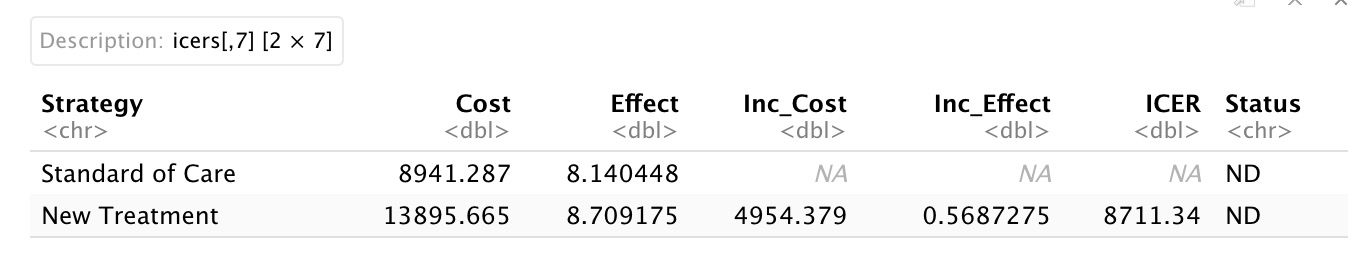
A table containing the cost-effectiveness results

The new treatment is cost-effective below a willingness-to-pay threshold of $8711.34 per QALY. This deterministic version of the model doesn’t allow us to examine the impact of parameter uncertainty. In order to do that we’ll need to make it probabilistic, which we will do in Step 3.

Back to Step 1

Back to top

You’ll notice that I am specifying the discount factor within this step rather than drawing it from the table itself like we did in the Batch Importer example. This is really just a matter of personal choice and comfort. If you are expecting people to use the model without having to touch the code, you will have to define ‘v_dwe’ and ‘v_dwc’ after you run the Batch Importer. ↩